
[This post was written by Dipanjan. Dipanjan works in the Engineering Team with Mandar, addressing some of the problems related to Data Semantics. He loves watching English Sitcoms in his spare time. This was originally posted on the PriceWeave blog.]
This is the second post in our series of blog posts which we shall be presenting regarding social media analysis. We have already talked about Twitter Mining in depth earlier and also how to analyze social trends in general and gather insights from YouTube. If you are more interested in developing a quick sentiment analysis app, you can check our short tutorial on that as well.
Our flagship product, PriceWeave, is all about delivering real time actionable insights at scale. PriceWeave helps Retailers and Brands take decisions on product pricing, promotions, and assortments on a day to day basis. One of the areas we focus on is “Social Intelligence”, where we measure our customers’ social presence in terms of their reach and engagement on different social channels. Social Intelligence also helps in discovering brands and products trending on social media.
Today, I will be talking about how we can get data from Twitter in real-time and perform some interesting analytics on top of that to understand social reactions to trending brands and products.
In our last post, we had used Twitter’s Search API for getting a selective set of tweets and performed some analytics on that. But today, we will be using Twitter’s Streaming API, to access data feeds in real time. A couple of differences with regards to the two APIs are as follows. The Search API is primarily a REST API which can be used to query for “historical data”. However, the Streaming API gives us access to Twitter’s global stream of tweets data. Moreover, it lets you acquire much larger volumes of data with keyword filters in real-time compared to normal search.
Installing Dependencies
I will be using Python for my analysis as usual, so you can install it if you don’t have it already. You can use another language of your choice, but remember to use the relevant libraries of that language. To get started, install the following packages, if you don’t have them already. We use simplejson for JSON data processing at DataWeave, but you are most welcome to use the stock json library.
Acquiring Data
We will use the Twitter Streaming API and the equivalent python wrapper to get the required tweets. Since we will be looking to get a large number of tweets in real time, there is the question of where should we store the data and what data model should be used. In general, when building a robust API or application over Twitter data, MongoDB being a schemaless document-oriented database, is a good choice. It also supports expressive queries with indexing, filtering and aggregations. However, since we are going to analyze a relatively small sample of data using pandas, we shall be storing them in flat files.
Note: Should you prefer to sink the data to MongoDB, the mongoexportcommand line tool can be used to export it to a newline delimited format that is exactly the same as what we will be writing to a file.
The following code snippet shows you how to create a connection to Twitter’s Streaming API and filter for tweets containing a specific keyword. For simplicity, each tweet is saved in a newline-delimited file as a JSON document. Since we will be dealing with products and brands, I have queried on two trending products and brands respectively. They are, ‘Sony’ and ‘Microsoft’ with regards to brands and ‘iPhone 6’ and ‘Galaxy S5’ with regards to products. You can write the code snippet as a function for ease of use and call it for specific queries to do a comparative study.
Let the data stream for a significant period of time so that you can capture a sizeable sample of tweets.
Analyses and Visualizations
Now that you have amassed a collection of tweets from the API in a newline delimited format, let’s start with the analyses. One of the easiest ways to load the data into pandas is to build a valid JSON array of the tweets. This can be accomplished using the following code segment.
Note: With pandas, you will need to have an amount of working memory proportional to the amount of data that you’re analyzing.
Once you run this, you should get a dictionary containing 4 data frames. The output I obtained is shown in the snapshot below.
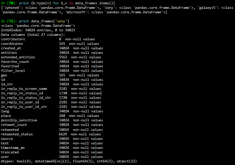
Note: Per the Streaming API guidelines, Twitter will only provide up to 1% of the total volume of real time tweets, and anything beyond that is filtered out with each “limit notice”.
The next snippet shows how to remove the “limit notice” column if you encounter it.
Time-based Analysis
Each tweet we captured had a specific time when it was created. To analyze the time period when we captured these tweets, let’s create a time-based index on the created_at field of each tweet so that we can perform a time-based analysis to see at what times do people post most frequently about our query terms.
The output I obtained is shown in the snapshot below.
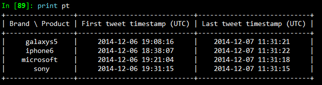
I had started capturing the Twitter stream at around 7 pm on the 6th of December and stopped it at around 11:45 am on the 7th of December. So the results seem consistent based on that. With a time-based index now in place, we can trivially do some useful things like calculate the boundaries, compute histograms and so on. Operations such as grouping by a time unit are also easy to accomplish and seem a logical next step. The following code snippet illustrates how to group by the “hour” of our data frame, which is exposed as a datetime.datetime timestamp since we now have a time-based index in place. We print an hourly distribution of tweets also just to see which brand \ product was most talked about on Twitter during that time period.
The outputs I obtained are depicted in the snapshot below.
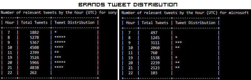
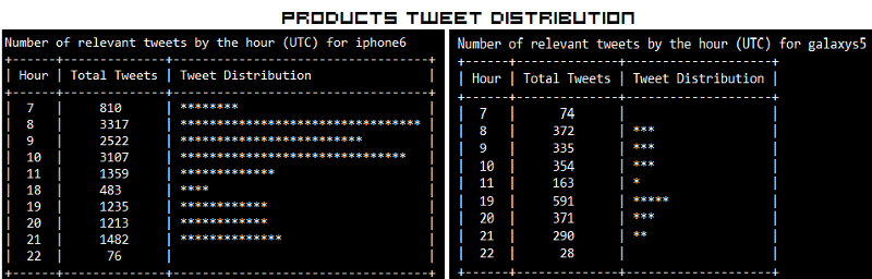
The “Hour” field here follows a 24 hour format. What is interesting here is that, people have been talking more about Sony than Microsoft in Brands. In Products, iPhone 6 seems to be trending more than Samsung’s Galaxy S5. Also the trend shows some interesting insights that people tend to talk more on Twitter in the morning and late evenings.
Time-based Visualizations
It could be helpful to further subdivide the time ranges into smaller intervals so as to increase the resolution of the extremes. Therefore, let’s group into a custom interval by dividing the hour into 15-minute segments. The code is pretty much the same as before except that you call a custom function to perform the grouping. This time, we will be visualizing the distributions using matplotlib.
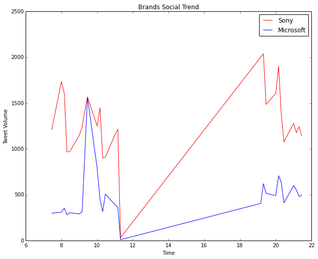
The two visualizations are depicted below. Of course don’t forget to ignore the section of the plots from after 11:30 am to around 7 pm because during this time no tweets were collected by me. This is indicated by a steep rise in the curve and is insignificant. The real regions of significance are from hour 7 to 11:30 and hour 19 to 22.
Considering brands, the visualization for Microsoft vs. Sony is depicted below. Sony is the clear winner here.
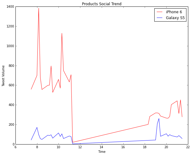
Considering products, the visualization for iPhone 6 vs. Galaxy S5 is depicted below. The clear winner here is definitely iPhone 6.
Tweeting Frequency Analysis
In addition to time-based analysis, we can do other types of analysis as well. The most popular analysis in this case would be frequency based analysis of the users authoring the tweets. The following code snippet will compute the Twitter accounts that authored the most tweets and compare it to the total number of unique accounts that appeared for each of our query terms.
The results which I obtained are depicted below.
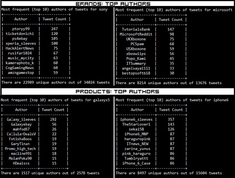
What we do notice is that a lot of these tweets are also made by bots, advertisers and SEO technicians. Some examples are Galaxy_Sleeves and iphone6_sleeves which are obviously selling covers and cases for the devices.
Tweeting Frequency Visualizations
After frequency analysis, we can plot these frequency values to get better intuition about the underlying distribution, so let’s take a quick look at it using histograms. The following code snippet created these visualizations for both brands and products using subplots.
The visualizations I obtained are depicted below.
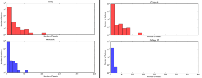
The distributions follow the “Pareto Principle” as expected where we see that a selective number of users make a large number of tweets and the majority of users create a small number of tweets. Besides that, we see that based on the tweet distributions, Sony and iPhone 6 are more trending than their counterparts.
Locale Analysis
Another important insight would be to see where your target audience is located and their frequency. The following code snippet achieves the same.
The outputs which I obtained are depicted in the following snapshot. Remember that Twitter follows the ISO 639–1 language code convention.
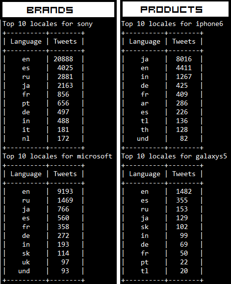
The trend we see is that most of the tweets are from English speaking countries as expected. Surprisingly, most of the Tweets regarding iPhone 6 are from Japan!
Analysis of Trending Topics
In this section, we will see some of the topics which are associated with the terms we used for querying Twitter. For this, we will be running our analysis on the tweets where the author speaks in English. We will be using the nltklibrary here to take care of a couple of things like removing stopwords which have little significance. Now I will be doing the analysis here for brands only, but you are most welcome to try it out with products too because, the following code snippet can be used to accomplish both the computations.
What the above code does is that, it takes each tweet, tokenizes it and then computes a term frequency and outputs the 20 most common terms for each brand. Of course an n-gram analysis can give a deeper insight into trending topics but the same can also be accomplished with ntlk’s collocations function which takes in the tokens and outputs the context in which they were mentioned. The outputs I obtained are depicted in the snapshot below.
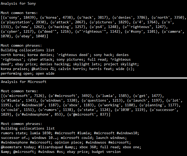
Some interesting insights we see from the above outputs are as follows.
- Sony was hacked recently and it was rumored that North Korea was responsible for that, however they have denied that. We can see that is trending on Twitter in context of Sony. You can read about it here.
- Sony has recently introduced Project Sony Skylight which lets you customize your PS4.
- There are rumors of Lumia 1030, Microsoft’s first flagship phone.
- People are also talking a lot about Windows 10, the next OS which is going to be released by Microsoft pretty soon.
- Interestingly, “ebay price” comes up for both the brands, this might be an indication that eBay is offering discounts for products from both these brands.
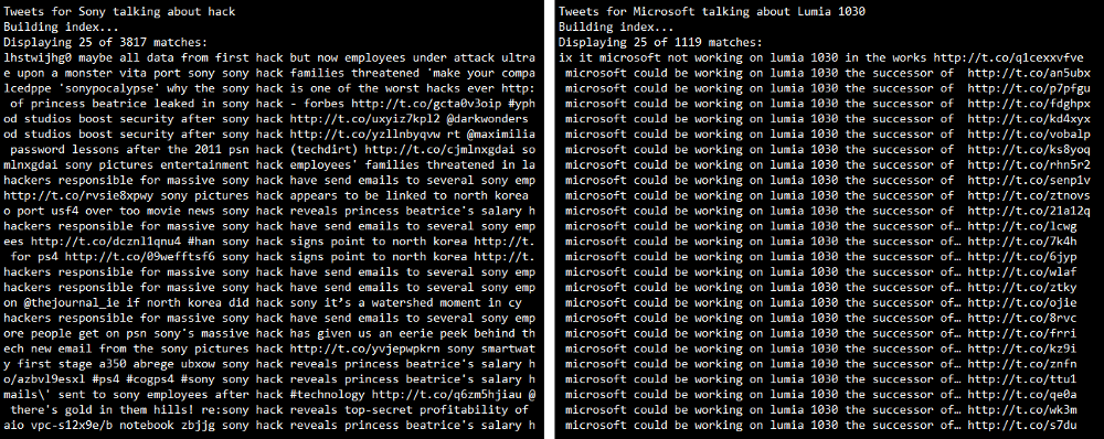
To get a detailed view on the tweets matching some of these trending terms, we can use nltk’s concordance function as follows.
The outputs I obtained are as follows. We can clearly see the tweets which contain the token we searched for. In case you are unable to view the text clearly, click on the image to zoom.
Thus, you can see that the Twitter Streaming API is a really good source to track social reaction to any particular entity whether it is a brand or a product. On top of that, if you are armed with an arsenal of Python’s powerful analysis tools and libraries, you can get the best insights from the unending stream of tweets.
That’s all for now folks! Before I sign off, I would like to thank Matthew A. Russell and his excellent book Mining the Social Web once again, without which this post would not have been possible. Cover image credit goes to TechCrunch.


Book a Demo
Login
For accounts configured with Google ID, use Google login on top.
For accounts using SSO Services, use the button marked "Single Sign-on".